Understanding the Vision Transformer: A New Era in Image Classification

In the rapidly evolving field of deep learning, the Vision Transformer (ViT) has emerged as a groundbreaking architecture for image classification. This article aims to provide a concise overview of the minor modifications made to the traditional transformer architecture to adapt it for image classification tasks. If you’re unfamiliar with the foundational concepts of transformers and attention mechanisms, I recommend checking out my previous articles on Transformers and Attention.

The Challenge with Traditional Transformers

Transformers, while powerful in natural language processing, lack certain inductive biases that Convolutional Neural Networks (CNNs) possess. Specifically, CNNs are designed with translation invariance and a locally restricted receptive field, allowing them to recognize objects in images regardless of their position or appearance. In contrast, transformers are permutation invariant and require sequential data for processing. This necessitates a transformation of spatial, non-sequential signals into a sequence format suitable for transformers.

How the Vision Transformer Works

The Vision Transformer (ViT) architecture can be broken down into several key steps:

1. Split an Image into Patches: The input image is divided into smaller, non-overlapping patches.
2. Flatten the Patches: Each patch is flattened into a one-dimensional vector.
3. Produce Linear Embeddings: The flattened patches are transformed into lower-dimensional linear embeddings.
4. Add Positional Embeddings: Positional information is added to the embeddings to retain spatial relationships.
5. Feed the Sequence into a Transformer Encoder: The sequence of embeddings is then processed through a standard transformer encoder.
6. Pretrain on Large Datasets: The model is pretrained on a large dataset with image labels.
7. Fine-tune on Downstream Tasks: Finally, the model is fine-tuned on specific datasets for image classification tasks.

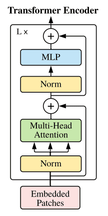
The encoder block used in ViT mirrors the original transformer architecture proposed by Vaswani et al. in 2017. The primary difference lies in the number of transformer blocks utilized, which can be adjusted based on the dataset size and complexity.

Key Modifications and Considerations

Data Requirements

One of the critical findings in the development of ViT is that it requires a substantial amount of data to perform effectively. Specifically, training on datasets with over 14 million images can enable ViT to rival or surpass the performance of state-of-the-art CNNs. For smaller datasets, traditional architectures like ResNets or EfficientNets may be more suitable.

Fine-tuning and Resolution

ViT is pretrained on large datasets and then fine-tuned on smaller ones. During fine-tuning, it is advantageous to work with higher resolutions than those used during pretraining. This is achieved through 2D interpolation of the pretrained positional embeddings, which are modeled using trainable linear layers.

Representing Images as Sequences

To convert an image into a sequence of patches, we start with an input image of dimensions ( H \times W \times C ) (height, width, and channels). Given a patch size ( P ), we create ( N ) image patches represented as ( N \times (P^2 \times C) ). The sequence length ( N ) is calculated as ( \frac{H \times W}{P^2} ).

Using the einops library, we can easily reshape the image into patches with the following code:

from einops import rearrange

p = patch_size
x_p = rearrange(img, 'b c (h p1) (w p2) -> b (h w) (p1 p2 c)', p1=p, p2=p)

Positional Embeddings

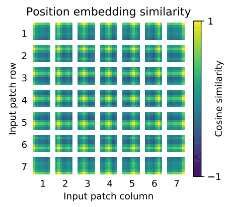
While various positional embedding schemes have been explored, no significant differences in performance have been observed. This is likely due to the transformer encoder’s operation at the patch level, making it easier to learn relationships between patches than between individual pixels. After the linear projection, a trainable positional embedding is added to the patch representations.

Key Findings and Insights

Attention Mechanism

One of the most intriguing aspects of ViT is its attention mechanism. Unlike CNNs, which require multiple layers to capture distant pixel interactions, ViT can learn non-local interactions from the very first layer. This is due to the self-attention mechanism, which allows the model to consider the entire patch during the initial processing stages.

Visualization of Learned Features

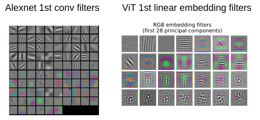
Visualizing the learned filters in ViT reveals a stark contrast to traditional CNNs. While CNNs often exhibit smooth and clustered features, ViT’s learned representations can be more complex and varied.

Attention Distance

The mean attention distance in ViT is analogous to the receptive field in CNNs. It measures the average distance between a query pixel and the rest of the patch, weighted by the attention score. This allows the model to focus on semantically relevant regions of the image for classification.

Implementation

For those interested in implementing ViT, here’s a simplified version of the code:

import torch
import torch.nn as nn
from einops import rearrange

class ViT(nn.Module):
    def __init__(self, img_dim, in_channels=3, patch_dim=16, num_classes=10, dim=512, blocks=6, heads=4, dim_linear_block=1024, dropout=0):
        super().__init__()
        assert img_dim % patch_dim == 0, f'patch size {patch_dim} not divisible'
        self.p = patch_dim
        tokens = (img_dim // patch_dim) ** 2
        self.token_dim = in_channels * (patch_dim ** 2)
        self.dim = dim
        self.project_patches = nn.Linear(self.token_dim, dim)
        self.emb_dropout = nn.Dropout(dropout)
        self.pos_emb1D = nn.Parameter(torch.randn(tokens, dim))
        self.transformer = TransformerEncoder(dim, blocks=blocks, heads=heads)

    def forward(self, img):
        batch_size = img.shape[0]
        img_patches = rearrange(img, 'b c (patch_x x) (patch_y y) -> b (x y) (patch_x patch_y c)', patch_x=self.p, patch_y=self.p)
        img_patches = self.project_patches(img_patches)
        patch_embeddings = self.emb_dropout(img_patches + self.pos_emb1D)
        return self.transformer(patch_embeddings)

Conclusion

The Vision Transformer represents a significant advancement in the field of image classification by framing the problem as a sequential task using image patches as tokens. While the architecture is elegant and effective, it requires substantial data and computational resources for optimal performance. As the field continues to evolve, the insights gained from ViT will undoubtedly influence future developments in computer vision.

For those looking to dive deeper into deep learning, consider exploring my book on building, training, and deploying deep learning models.

Disclosure: Some links in this article may be affiliate links, and at no additional cost to you, I may earn a commission if you decide to make a purchase after clicking through.