Unraveling the Mysteries of Recurrent Neural Networks: A Comprehensive Guide

In the realm of artificial intelligence, particularly within the computer vision community, recurrent neural networks (RNNs) often evoke a sense of mystery. Many practitioners find themselves in desperate situations, grappling with the complexities of these models without a clear understanding of their inner workings. RNNs, much like a black box, can be intimidating, but fear not! This tutorial aims to demystify RNNs, particularly focusing on Long Short-Term Memory (LSTM) networks, and provide a modern guide to their practical applications.

The Importance of Understanding RNNs

RNNs are pivotal in various applications, including sequence prediction, activity recognition, video classification, and natural language processing tasks. However, the abstraction of RNN implementations often obscures the underlying mechanics, making it challenging for users to grasp how time dimensions are handled in sequences. As Andrey Karpathy, Director of AI at Tesla, aptly stated, “If you insist on using the technology without understanding how it works, you are likely to fail.” This tutorial seeks to bridge that gap, empowering you to write optimized code and practice extensibility with confidence.

A Simple RNN Cell

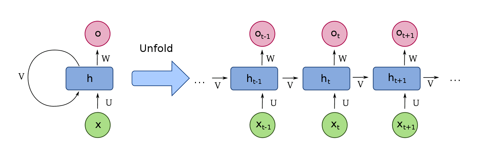
At its core, a recurrent cell is a neural network designed for processing sequential data. Unlike convolutional layers, which are tailored for grid-structured data like images, recurrent layers are adept at handling long sequences without requiring additional sequence-based design choices. This is achieved by connecting the outputs of previous timesteps to the inputs of the current timestep—a process known as sequence unrolling. This connection introduces the concept of memory, allowing the model to retain information from prior states.

Visualization of an RNN Cell

The above visualization illustrates how RNN cells can process sequences of variable lengths, making them suitable for applications like video analysis, where the number of frames may vary. By sharing weights across multiple timesteps, RNNs can effectively utilize previous states to inform current predictions.

Training RNNs: Backpropagation Through Time

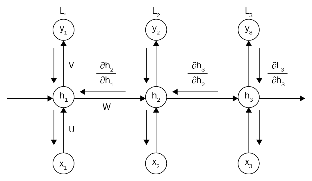
Understanding how to train RNNs is crucial, especially for those with a background in computer vision. The concept of Backpropagation Through Time (BPTT) is fundamental to training RNNs. This technique involves unrolling the RNN through time, allowing for the calculation of gradients across multiple timesteps.

When training an RNN, we aim to learn temporal dependencies, which is something traditional convolutional networks struggle with due to their finite receptive fields. BPTT enables us to compute gradients from multiple paths (timesteps), which are then aggregated to update the model’s parameters. This process is essential for learning long-term dependencies in sequential data.

Visualization of BPTT

The image above illustrates how BPTT operates by calculating losses at each timestep and backpropagating the errors to the memory cells. This method allows RNNs to learn from the entire sequence, making them powerful tools for tasks involving time-series data.

LSTM: Long Short-Term Memory Cells

Why LSTM?

LSTMs were introduced to address the limitations of standard RNNs, particularly their inability to learn long-term dependencies effectively. Research by Greff et al. (2016) demonstrated that LSTMs consistently outperform other RNN variations in large-scale studies, solidifying their status as the dominant architecture in the field.

How LSTM Works

LSTMs utilize a more complex architecture than standard RNNs, incorporating three gates: the input gate, forget gate, and output gate. These gates regulate the flow of information, allowing the LSTM to retain or discard information as needed.

Equations of the LSTM Cell

1. Input Gate:
   [
   it = \sigma(W{xi} xt + W{hi} h_{t-1} + b_i)
   ]
2. Forget Gate:
   [
   ft = \sigma(W{xf} xt + W{hf} h_{t-1} + b_f)
   ]
3. Cell State Update:
   [
   c_t = ft \odot c{t-1} + it \odot \tanh(W{xc} xt + W{hc} h_{t-1} + b_c)
   ]
4. Output Gate:
   [
   ot = \sigma(W{xo} xt + W{ho} h_{t-1} + b_o)
   ]
5. Hidden State:
   [
   h_t = o_t \odot \tanh(c_t)
   ]

These equations encapsulate the LSTM’s ability to manage information over time, allowing it to learn from both recent and distant past inputs effectively.

Implementing a Custom LSTM Cell in PyTorch

With a solid understanding of LSTM mechanics, let’s implement a custom LSTM cell in PyTorch. This implementation will simplify the original LSTM architecture while maintaining its core functionalities.

import torch
from torch import nn

class LSTMCellCustom(nn.Module):
    def __init__(self, input_size, hidden_size):
        super(LSTMCellCustom, self).__init__()
        self.input_size = input_size
        self.hidden_size = hidden_size

        self.W_f = nn.Linear(input_size + hidden_size, hidden_size)
        self.W_i = nn.Linear(input_size + hidden_size, hidden_size)
        self.W_c = nn.Linear(input_size + hidden_size, hidden_size)
        self.W_o = nn.Linear(input_size + hidden_size, hidden_size)

    def forward(self, x, hidden):
        h_prev, c_prev = hidden

        combined = torch.cat((x, h_prev), 1)
        f_t = torch.sigmoid(self.W_f(combined))
        i_t = torch.sigmoid(self.W_i(combined))
        c_t = f_t * c_prev + i_t * torch.tanh(self.W_c(combined))
        o_t = torch.sigmoid(self.W_o(combined))
        h_t = o_t * torch.tanh(c_t)

        return h_t, c_t

This custom implementation captures the essence of LSTM cells while allowing for educational exploration and experimentation.

Connecting LSTM Cells Across Time and Space

LSTM cells can be connected both temporally and spatially. In a temporal context, we can visualize a sequence of LSTM cells processing inputs over time. In a spatial context, we can stack multiple LSTM layers, where the output of one layer serves as the input to the next.

Example of Temporal Connection

In a simple sequence of N timesteps, each LSTM cell processes its corresponding input and passes its hidden state to the next cell, effectively unrolling the sequence.

Example of Spatial Connection

When stacking LSTM layers, the output of the first layer becomes the input to the second layer. This hierarchical structure allows for more complex representations and learning.

Validation: Learning a Sine Wave with an LSTM

To validate our custom LSTM implementation, we can use a simple task: predicting values of a sine wave. By replacing the standard LSTM cell in a PyTorch example with our custom implementation, we can observe how well it performs.

Results

Upon running the modified code, we can visualize the predicted sine wave values against the actual values, confirming the correctness of our implementation. This exercise not only serves as a sanity check but also reinforces our understanding of LSTM mechanics.

Bidirectional LSTM

An extension of the LSTM architecture is the Bidirectional LSTM, which processes input sequences in both forward and backward directions. This approach can be beneficial in tasks where context from both ends of the sequence is valuable.

Considerations for Bidirectional LSTM

Before implementing a bidirectional LSTM, consider whether your task benefits from learning temporal correlations in both directions. Keep in mind that this approach doubles the number of parameters and the output vector size.

Conclusion

In summary, recurrent neural networks, particularly LSTMs, are powerful tools for modeling sequential data. By understanding their inner workings, we can leverage their capabilities to tackle complex tasks involving time-varying data. This tutorial has provided a comprehensive overview of RNNs, from basic concepts to practical implementation, empowering you to explore this fascinating area of deep learning with confidence.

For further exploration, consider diving into TensorFlow tutorials on text generation with RNNs or exploring advanced topics such as GRU cells. The journey into the world of recurrent neural networks is just beginning, and the possibilities are endless!