A Hands-On Tutorial on Medical Imaging: Understanding Computed Tomography (CT) with Basic Image Processing Algorithms
In the realm of medical imaging, Computed Tomography (CT) stands out as a powerful tool for visualizing the internal structures of the human body. While deep learning and advanced AI techniques have gained significant traction in recent years, it is crucial for practitioners to grasp the foundational concepts of image processing. This article aims to provide a comprehensive, hands-on tutorial on CT imaging, utilizing basic image processing algorithms to segment and analyze lung areas and blood vessels.
Introduction to CT Imaging
The Physics of CT Scans
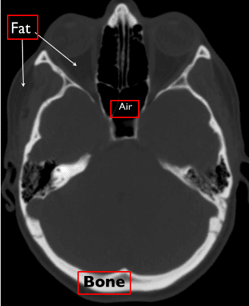
Computed Tomography employs X-ray beams to capture 3D pixel intensities of the human body. The process begins with a heated cathode that releases high-energy electrons, which then emit X-ray radiation. As these X-rays traverse the body, they interact with various tissues, with denser tissues (like bones) absorbing more radiation than softer tissues (like fat). This differential absorption creates a contrast that allows us to visualize internal structures. Areas where X-rays pass through without absorption appear black (like air in the lungs), while denser tissues appear white.

CT Intensities and Hounsfield Units
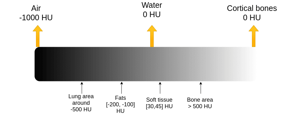
The absorption of X-rays is quantified using the Hounsfield scale, where air is assigned a value of -1000 and water is set at 0. Unlike MRI, which uses a relative scale from 0 to 255, the Hounsfield scale is absolute. Understanding this scale is vital for interpreting CT images, as it provides insight into the density of various tissues.

CT Data Visualization: Level and Window
To visualize CT data effectively, we utilize a technique known as "windowing," which involves selecting a central intensity (level) and a range (window) around it. This allows us to focus on specific tissues while ignoring irrelevant data. The following code snippet demonstrates how to implement this in Python:
import matplotlib.pyplot as plt
import numpy as np

def show_slice_window(slice, level, window):
    """Function to display an image slice."""
    max_val = level + window / 2
    min_val = level - window / 2
    slice = slice.clip(min_val, max_val)
    plt.figure()
    plt.imshow(slice.T, cmap="gray", origin="lower")
    plt.savefig('L'+str(level)+'W'+str(window))
Lung Segmentation Based on Intensity Values
In this section, we will segment the lungs from a CT image and calculate their area in mm². The process involves several steps:
Step 1: Find Pixel Dimensions
To accurately calculate the area, we first need to extract the pixel dimensions from the CT image header. This can be done using the nibabel library:
import nibabel as nib

ct_img = nib.load(exam_path)
print(ct_img.header)
Step 2: Binarize Image Using Intensity Thresholding
Next, we will binarize the image based on the expected Hounsfield unit range for the lungs, which is typically between -1000 and -300. This step involves clipping the image and converting it to a binary mask:
def intensity_seg(ct_numpy, min=-1000, max=-300):
    clipped = clip_ct(ct_numpy, min, max)
    return measure.find_contours(clipped, 0.95)
Step 3: Contour Finding
Using the marching squares method from the skimage library, we can identify contours in the binary mask:
from skimage import measure

contours = measure.find_contours(clipped, 0.95)
Step 4: Find the Lung Area from Contours
To isolate the lung areas, we can apply constraints to exclude non-lung regions. This involves analyzing the contours and selecting those that correspond to the lungs:
def find_lungs(contours):
    body_and_lung_contours = []
    vol_contours = []
    for contour in contours:
        hull = ConvexHull(contour)
        if hull.volume > 2000 and set_is_closed(contour):
            body_and_lung_contours.append(contour)
            vol_contours.append(hull.volume)
    # Further processing to exclude body contours...
Step 5: Contour to Binary Mask
Finally, we convert the identified contours into a binary mask, which can be saved in the NIfTI format for further analysis:
def create_mask_from_polygon(image, contours):
    lung_mask = np.array(Image.new('L', image.shape, 0))
    for contour in contours:
        x = contour[:, 0]
        y = contour[:, 1]
        polygon_tuple = list(zip(x, y))
        img = Image.new('L', image.shape, 0)
        ImageDraw.Draw(img).polygon(polygon_tuple, outline=0, fill=1)
        mask = np.array(img)
        lung_mask += mask
    lung_mask[lung_mask > 1] = 1
    return lung_mask.T
Segmenting Main Vessels and Computing the Vessels Over Lung Area Ratio
To identify blood vessels within the lung area, we can apply a similar approach. Pixels with intensity values greater than -500 HU are considered vessels. The following function illustrates this process:
def create_vessel_mask(lung_mask, ct_numpy):
    vessels = lung_mask * ct_numpy
    vessels[vessels == 0] = -1000
    vessels[vessels >= -500] = 1
    vessels[vessels < -500] = 0
    return vessels
Conclusion and Further Readings
This tutorial has provided a foundational understanding of CT imaging and basic image processing techniques for lung segmentation and vessel analysis. By mastering these concepts, practitioners can better appreciate the capabilities and limitations of deep learning in medical imaging.
For those interested in furthering their knowledge, I recommend exploring the following resources:
You can access the accompanying Google Colab notebook here and the GitHub repository for the code used in this tutorial.
By engaging with these materials, you will be well-equipped to navigate the exciting field of medical imaging, whether through traditional image processing techniques or advanced AI methodologies. Happy coding!
