Understanding Input Scaling in Machine Learning: A Comprehensive Guide to Normalization Methods
When delving into the world of machine learning, one of the first concepts you encounter is input scaling, particularly normalization. The importance of this concept cannot be overstated, especially when training models using gradient descent. Training a model with non-normalized features can lead to suboptimal performance, as the model may inadvertently ignore certain features due to their differing scales. In this article, we will explore the various normalization methods available, their applications, and the rationale behind their use.
Why Normalize?
To grasp the necessity of normalization, consider a simple yet illustrative example. Imagine two input features: one ranges from [0, 1], while the other spans [0, 10,000]. In this scenario, the model may overlook the first feature entirely, as its weight is initialized in a small range. This issue is compounded by the potential for exploding gradients, which can further destabilize the training process.
This challenge is not limited to the input layer; it extends to the layers of deep neural networks, regardless of architecture—be it transformers, convolutional neural networks (CNNs), recurrent neural networks (RNNs), or generative adversarial networks (GANs). Each intermediate layer functions similarly to the input layer, accepting features and transforming them. Therefore, effective normalization techniques are essential for enhancing training efficiency, performance, and stability.
Trends in Normalization Methods
As machine learning has evolved, various normalization methods have emerged, each tailored for specific tasks and architectures. Below is a graph illustrating the trends in normalization methods used across different research papers over time:

For those seeking a deeper understanding of deep learning fundamentals, we recommend the Coursera specialization.
Notations
Throughout this article, we will use the following notations:
- ( N ): Batch size
- ( H ): Height
- ( W ): Width
- ( C ): Feature channels
- ( \mu ): Mean
- ( \sigma ): Standard deviation
- ( x, y, m \in \mathbb{R}^{N \times C \times H \times W} ): Batch features
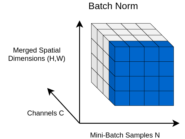
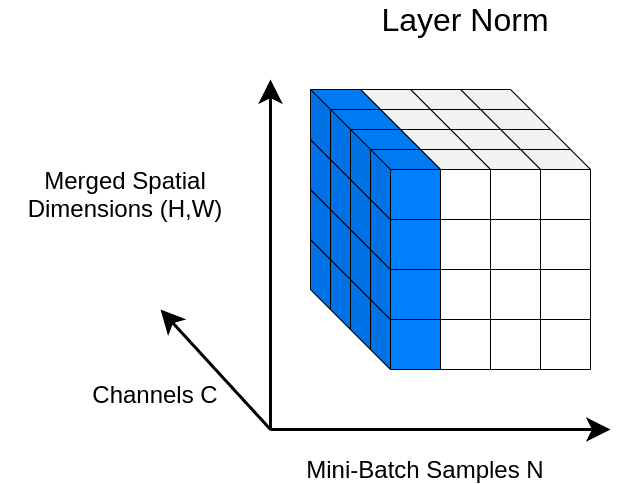
We will also visualize the 4D activation maps ( x ) by merging the spatial dimensions into a 3D shape.

Common Normalization Methods
1. Batch Normalization (2015)
Batch Normalization (BN) is a widely adopted technique that normalizes the mean and standard deviation for each individual feature channel or map. By ensuring that the features follow a Gaussian distribution with zero mean and unit variance, BN effectively brings the features into a compact range.
Mathematically, BN can be expressed as:
[
BN(x) = \gamma\left(\frac{x – \mu(x)}{\sigma(x)}\right) + \beta
]
Where:
- ( \mu_c(x) ) and ( \sigma_c(x) ) are the mean and standard deviation calculated over the batch.

Advantages of Batch Normalization:
- Accelerates training of deep networks.
- Introduces a form of regularization, reducing internal covariate shift.
- Improves gradient flow, allowing for higher learning rates.
Disadvantages:
- Inaccurate estimation of batch statistics with small batch sizes.
- Issues arise when batch sizes vary between training and inference.
2. Synchronized Batch Normalization (2018)
As training scales increased, Synchronized Batch Normalization (Synch BN) was developed. Unlike standard BN, which updates mean and variance separately for each GPU, Synch BN communicates these statistics across multiple workers.
3. Layer Normalization (2016)
Layer Normalization (LN) computes statistics across all channels and spatial dimensions, making it independent of batch size. This method is particularly useful for handling vectors, such as RNN outputs.
Mathematically, LN is defined as:
[
LN(x) = \gamma\left(\frac{x – \mu(x)}{\sigma(x)}\right) + \beta
]
Where the mean and variance are computed across all channels and spatial dimensions.

4. Instance Normalization (2016)
Instance Normalization (IN) normalizes features across spatial dimensions independently for each channel and sample. This method is particularly effective in style transfer applications, allowing for the manipulation of individual styles.
5. Weight Normalization (2016)
Weight Normalization reparameterizes the weights of a layer, separating the magnitude from its direction. This technique aims to accelerate training by smoothing the optimization landscape.
6. Adaptive Instance Normalization (2017)
Adaptive Instance Normalization (AdaIN) aligns the channel-wise mean and variance of a content image to match those of a style image, enabling effective style transfer.
7. Group Normalization (2018)
Group Normalization divides channels into groups and computes statistics within each group, making it independent of batch sizes and providing more stable accuracy across varying batch sizes.
8. Weight Standardization (2019)
Weight Standardization builds upon Weight Normalization by controlling the first-order statistics of the weights of each output channel individually, further smoothing the loss landscape.
9. SPADE (2019)
SPADE (Spatially-Adaptive Normalization) extends the idea of AdaIN by incorporating segmentation maps, allowing for more consistent image synthesis.
Conclusion
Normalization methods play a crucial role in the training of deep neural networks, enhancing performance and stability. From Batch Normalization to SPADE, each method has its unique advantages and applications. Understanding these techniques is essential for anyone looking to excel in the field of machine learning.
If you found this article informative, consider sharing it on your social media to help others learn about the importance of normalization in machine learning!
References
- Ioffe, S., & Szegedy, C. (2015). Batch normalization: Accelerating deep network training by reducing internal covariate shift.
- Salimans, T., & Kingma, D. P. (2016). Weight normalization: A simple reparameterization to accelerate training of deep neural networks.
- Ba, J. L., Kiros, J. R., & Hinton, G. E. (2016). Layer normalization.
- Ulyanov, D., Vedaldi, A., & Lempitsky, V. (2016). Instance normalization: The missing ingredient for fast stylization.
- Wu, Y., & He, K. (2018). Group normalization.
- Zhang, H., et al. (2018). Context encoding for semantic segmentation.
- Santurkar, S., et al. (2018). How does batch normalization help optimization?.
- Dumoulin, V., et al. (2016). A learned representation for artistic style.
- Park, T., et al. (2019). Semantic image synthesis with spatially-adaptive normalization.
- Huang, X., & Belongie, S. (2017). Arbitrary style transfer in real-time with adaptive instance normalization.
- Kolesnikov, A., et al. (2019). Big transfer (BiT): General visual representation learning.
- Qiao, S., et al. (2019). Weight standardization.
