Understanding Graph Neural Networks and Graph Convolutions: A Beginner’s Guide
In this tutorial, we will delve into the fascinating world of Graph Neural Networks (GNNs) and graph convolutions. Graphs are a versatile representation of data that encapsulate intrinsic structures, making them a powerful tool in various domains. This article aims to clarify some of the more complex concepts for beginners in this field, starting from a familiar ground: images.
The Intuitive Transition from Images to Graphs
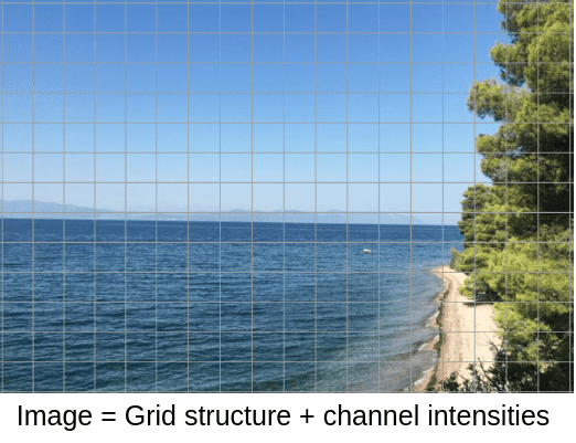
Why begin with images? Images are structured data where components (pixels) are arranged meaningfully. Altering the arrangement of pixels can lead to a loss of meaning, highlighting the importance of structure. Additionally, images exhibit a strong notion of locality, where neighboring pixels often share similar characteristics.

In an image, pixels are organized in a grid, emphasizing the significance of structure. This structure allows us to design filters that aggregate representations from neighboring pixels, a process known as convolutions. Each pixel can be represented by a vector of features, such as intensity channels in grayscale or RGB images.
The key takeaway here is the separation of structure and signal (features), which is crucial for understanding graphs.
Decomposing Features and Structure
Similar to images, natural language can also be decomposed into signal and structure. The structure in language is defined by the order of words, which conveys syntax and grammatical context. For instance, in a sentence, words can be represented as nodes, while their connections (order) can be encoded in positional embeddings.
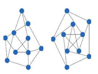
Graphs operate on the same principle: they consist of nodes (representing features) and edges (representing structure).
Real-World Signals That We Can Model with Graphs
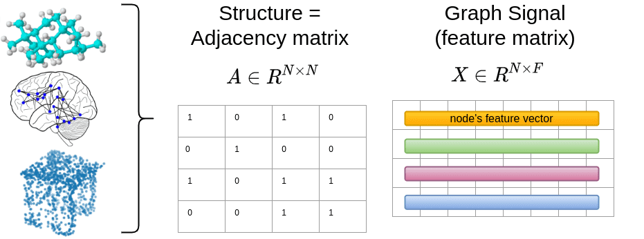
Graphs can model a wide array of real-world signals, provided we can define their structure and features. Formally, nodes are represented as (N), and the connectivity is defined by an (N \times N) adjacency matrix (A). The element (A_{ij}) indicates whether node (i) is connected to node (j).
The signal for each node can be represented as (X \in \mathbb{R}^{N \times F}), where (F) is the number of features. For example, an RGB image has (F=3) features, while a word might have a different embedding dimension.
Graphs can represent various data types, including brain graphs from medical imaging, social networks, point clouds, and molecular structures.

The Basic Mathematics for Processing Graph-Structured Data
To process graph-structured data, we need to understand some fundamental mathematical concepts. We have already defined the graph signal (X) and the adjacency matrix (A). An important feature is the degree of each node, which is the number of connections it has.
The degree vector can be calculated by summing the rows of the adjacency matrix (A). This degree vector can be placed in a diagonal (N \times N) matrix, known as the degree matrix (D).
import torch

a = torch.rand(3, 3)
a[a > 0.5] = 1
a[a <= 0.5] = 0

def calc_degree_matrix(a):
    return torch.diag(a.sum(dim=-1))

d = calc_degree_matrix(a)
The degree matrix (D) is fundamental in graph theory as it provides a single value for each node and is used to compute the graph Laplacian.
The Graph Laplacian
The graph Laplacian (L) is defined as:
[
L = D – A
]
In practice, we can compute the graph Laplacian using the following function:
def create_graph_lapl(a):
    return calc_degree_matrix(a) - a
The normalized version of the graph Laplacian is often used in graph neural networks to account for varying connectivity among nodes, which can lead to instabilities during training.
[
L_{norm} = D^{-\frac{1}{2}} L D^{-\frac{1}{2}} = I – D^{-\frac{1}{2}} A D^{-\frac{1}{2}}
]
This normalization ensures that the diagonal elements are ones when there is at least one connection, allowing for stable training.
Laplacian Eigenvalues and Eigenvectors
Eigenvalues and eigenvectors are crucial in understanding the properties of a graph. The zeroth eigenvalue indicates whether the graph is connected. If a graph has (k) connected components, the eigenvalue 0 has a multiplicity of (k).
For instance, consider a graph with two disconnected components; it would have two zero eigenvalues.

The smallest non-zero eigenvalue is particularly useful for spectral image segmentation, where we can divide an image based on its slowest frequencies.
How to Represent a Graph: Types of Graphs
Graphs can be classified into several types:
Directed vs. Undirected Graphs
Graphs can have directionality, which is reflected in the adjacency matrix. A symmetric (A) indicates an undirected graph, while a non-symmetric (A) denotes a directed graph.
Weighted vs. Unweighted Graphs
Graphs can also have weighted connections, where the adjacency matrix contains values other than binary indicators. This allows for more nuanced representations, such as distances between points in a point cloud.
The COO Format
The Coordinate Format (COO) is a common way to store sparse adjacency matrices, which is more efficient than storing the entire matrix.
Types of Graph Tasks: Graph and Node Classification
In graph neural networks, the primary tasks include:
- Graph Classification: Assigning a single label to an entire graph.
- Node Classification: Predicting labels for individual nodes within a graph, often in a semi-supervised manner.
How Graph Convolution Layers Are Formed
The principle behind graph convolutions is that convolution in the vertex domain corresponds to multiplication in the graph spectral domain. The simplest implementation of a graph neural network can be expressed as:
[
Y = (AX)W
]
Where (W) is a trainable parameter and (Y) is the output. This formulation allows us to account for both the signal (X) and the structure (A).
Implementing a 1-Hop GCN Layer in PyTorch
To illustrate the concepts discussed, we can implement a simple 1-hop Graph Convolutional Network (GCN) layer in PyTorch:
import torch
from torch import nn
import torch.nn.functional as F

class GCN_AISUMMER(nn.Module):
    def __init__(self, in_features, out_features, bias=True):
        super().__init__()
        self.linear = nn.Linear(in_features, out_features, bias=bias)

    def forward(self, X, A):
        L = create_graph_lapl_norm(A)
        x = self.linear(X)
        return torch.bmm(L, x)
Training Our GCN for Graph Classification
We can train our GCN on a dataset, such as the MUTAG dataset, to demonstrate its effectiveness. The architecture includes multiple GCN layers followed by a fully connected layer for classification.
class GNN(nn.Module):
    def __init__(self, in_features=7, hidden_dim=64, classes=2, dropout=0.5):
        super(GNN, self).__init__()
        self.conv1 = GCN_AISUMMER(in_features, hidden_dim)
        self.conv2 = GCN_AISUMMER(hidden_dim, hidden_dim)
        self.conv3 = GCN_AISUMMER(hidden_dim, hidden_dim)
        self.fc = nn.Linear(hidden_dim, classes)
        self.dropout = dropout

    def forward(self, x, A):
        x = self.conv1(x, A)
        x = F.relu(x)
        x = self.conv2(x, A)
        x = F.relu(x)
        x = self.conv3(x, A)
        x = F.dropout(x, p=self.dropout, training=self.training)
        x = x.mean(dim=1)
        return self.fc(x)
Conclusion
This tutorial provided a comprehensive introduction to Graph Neural Networks and graph convolutions, emphasizing the importance of understanding the separation of structure and signal. We explored the mathematical foundations, types of graphs, and practical implementations in PyTorch.
For those eager to dive deeper into the world of GNNs, I recommend exploring libraries like PyTorch Geometric, which offer extensive resources and tutorials.
If you found this article helpful, consider sharing it on social media to help spread accessible AI knowledge!
